How to Use Pivot Tables in Excel: A Complete Step-by-Step Guide

Working with large datasets in Excel can quickly become overwhelming. When numbers run into thousands of rows, simple sorting or filtering often fails to provide meaningful insights. This is where PivotTables—one of Excel’s most powerful analytical tools—step in. If you have ever wondered how professionals summarize huge datasets within seconds, the answer almost always involves PivotTables.

This guide explains How to Use Pivot Tables in Excel in a clear, structured, and human-friendly way. Whether you are a student, business owner, accountant, data analyst, or someone managing everyday spreadsheets, this tutorial will help you master PivotTables from the ground up.

PivotTables allow you to summarize, reorganize, analyze, and compare data with just a few clicks. You can calculate totals, averages, counts, percentages, performance comparisons, and more—without writing a single formula. The feature is widely used in reporting, financial modeling, sales tracking, HR dashboards, inventory analysis, and almost every industry that works with data.

This guide not only shows How to Use Pivot Tables in Excel, but also gives additional explanations, practical examples, troubleshooting tips, and real-world use cases so that you confidently use PivotTables like a pro.

Also Read: How to Set Up Auto HDR on Windows 11 for Gaming: Complete Step-by-Step Guide

---

Why PivotTables Matter: Understanding the Core Purpose

Before learning how to use Pivot Tables in Excel, it is important to understand why millions of Excel users depend on them. When data grows, normal spreadsheet methods become insufficient. For example:

• Counting sales per region manually is inefficient
• Calculating monthly profits using formulas requires constant editing
• Creating category-wise summaries becomes time-consuming
• Comparing performance across multiple segments is error-prone

A PivotTable solves these problems instantly. It dynamically reorganizes information so you can view it from different angles—much like rotating a physical object to see all sides. This “pivoting” action is what makes the tool extremely flexible.

Instead of writing multiple SUMIF, COUNTIF, or VLOOKUP formulas, you only:

1. Prepare data properly
2. Insert PivotTable
3. Arrange fields using drag-and-drop
4. Refresh when data changes

Everything else is automated.

---

1. Preparing Your Data for PivotTables

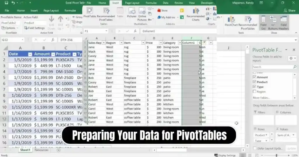
Learning How to Use Pivot Tables in Excel effectively begins with organizing your dataset. PivotTables work best when the underlying data is clean, consistent, and formatted properly.

Use a Tabular Structure

Your data should look like a structured table with:

• One unique header per column
• No merged cells in data
• No blank rows within the dataset

Each column should represent a single type of information, such as:

• Salesperson
• Region
• Product
• Quantity sold
• Sales amount
• Date

When data is arranged clearly, Excel automatically identifies patterns and makes pivoting easier.

Use Consistent Data Types

If a column contains numbers, avoid mixing text. If dates are included, ensure they truly register as dates—not text strings. PivotTables interpret values differently based on format, so consistency is essential.

Remove Blank Rows and Columns

Gaps may break the data range, causing incomplete PivotTables. Even a single blank row can cause Excel to stop reading beyond that point.

Convert Your Dataset Into an Excel Table (Highly Recommended)

One of the best practices in How to Use Pivot Tables in Excel is formatting your dataset as an Excel Table.

To do this:

• Select any cell inside the data
• Navigate to Insert > Table
• Confirm the range
• Check “My table has headers”
• Click OK

Benefits of using Excel Tables:

• Automatically expand when new data is added
• Ensures PivotTables refresh correctly
• Improves readability and structure
• Enables easy styling and filtering

These foundations make your upcoming PivotTable both stable and accurate.

---

2. How to Insert a PivotTable in Excel

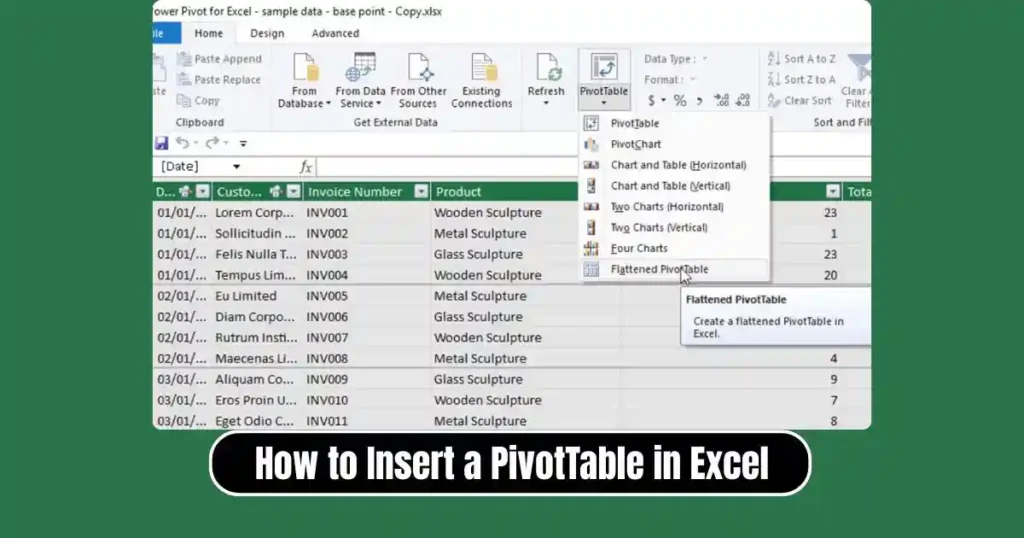
Now that your dataset is ready, the next step in How to Use Pivot Tables in Excel is creating the PivotTable itself.

Select a Cell Inside Your Data

This tells Excel which dataset you want to analyze. If your data is formatted as a table, Excel automatically selects the entire table.

Go to the Insert Tab

On the Excel ribbon, click Insert. Under this menu, locate the PivotTable button. Some versions also offer Recommended PivotTables, where Excel suggests several layout templates.

Click PivotTable

A dialog box appears.

Verify the Data Range

Excel usually detects your entire dataset correctly. But if necessary, you can manually adjust the range.

Choose Where to Place the PivotTable

You have two options:

• New Worksheet – Preferred for clarity
• Existing Worksheet – Useful for dashboards

Select OK to generate a blank PivotTable along with the PivotTable Fields pane on the right.

You have successfully created the platform where your analysis will happen.

---

3. Understanding the PivotTable Fields Pane

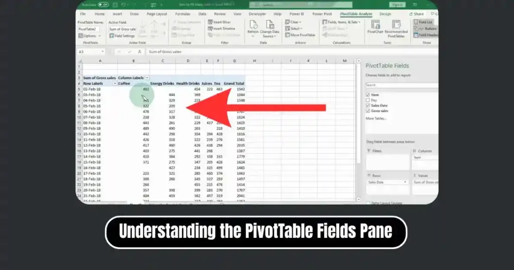
To master How to Use Pivot Tables in Excel, you must understand how the four analysis areas work:

Rows Area

• Creates row labels (categories)
• Example: List of salespersons, products, cities, or departments

Columns Area

• Creates column headings
• Useful for cross-tab comparisons
• Example: Product types across months

Values Area

• Performs calculations
• Common calculations: Sum, Average, Count, Max, Min

Filters Area

• Enables high-level filtering for the entire report
• Example: Filter by year, region, or manager

These four zones are the backbone of PivotTables.

---

4. How to Build a PivotTable Report: Practical Example

Let’s assume you have data containing:

• Salesperson names
• Products sold
• Regions
• Sales amount
• Dates

To see total sales per salesperson:

1. Drag Salesperson → Rows
2. Drag Sales Amount → Values

Excel immediately creates a summary showing each person’s contribution. This example highlights the beauty of PivotTables—instant summarization without formulas.

Another Example: Comparing Product Sales by Region

Drag fields as follows:

• Region → Columns
• Product → Rows
• Sales Amount → Values

This creates a matrix-like report displaying how each product performed across different regions.

Adjusting Calculations

Sometimes Excel defaults to Count instead of Sum. To change it:

1. Click the arrow next to the field in Values
2. Click Value Field Settings
3. Select:
   • Sum
   • Average
   • Count
   • Max
   • Min
   • Percentage calculations
4. Click OK

---

5. Sorting, Filtering, and Customizing the PivotTable

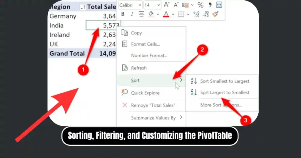
Once you understand How to Use Pivot Tables in Excel, you can fine-tune the report for deeper insights.

Sorting

Sort data from highest to lowest to identify top performers.
Right-click a row or column > Sort.

Filtering

Use built-in dropdowns to filter entries.
This is especially useful for:

• Showing only high-value customers
• Filtering specific date ranges
• Viewing only certain product categories

Grouping Data

Grouping allows you to analyze by:

• Months, quarters, years
• Numeric ranges
• Categories

To group dates:

1. Right-click a date field
2. Select Group
3. Choose Month/Quarter/Year

Also Read: How to Use Windows 11 Focus Sessions to Improve Productivity- Complete Guide

---

6. Refreshing the PivotTable After Data Changes

PivotTables do not update automatically when source data changes.

To refresh:

• Right-click anywhere inside the PivotTable
• Click Refresh

If you added new rows in an Excel Table, they automatically extend to the PivotTable upon refresh.

---

7. Advantages of Using PivotTables

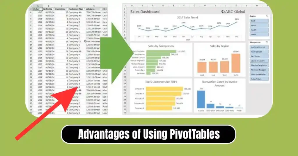
Understanding How to Use Pivot Tables in Excel unlocks several benefits:

Time Efficiency

PivotTables convert hours of manual work into seconds of automated analysis.

Error Reduction

Since calculations are automated, chances of human error drop drastically.

Flexible Analysis

You can rearrange fields anytime to explore new insights.

Customization Options

PivotTables support:

• Charts
• Conditional formatting
• Calculated fields
• Drill-down details

Industry-Wide Application

From finance to marketing to operations, PivotTables support all data-driven tasks.

---

8. Common Mistakes Beginners Make When Using PivotTables

Even after learning How to Use Pivot Tables in Excel, many users face issues. Common errors include:

• Using inconsistent data types
• Forgetting to refresh the PivotTable
• Not converting data into a Table
• Placing text fields in the Values area
• Using blank rows in data

Avoiding these mistakes improves accuracy and speed.

---

9. Real-World Use Cases of PivotTables

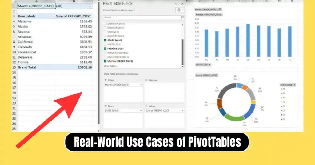
Sales Analysis

Track monthly revenue, salesperson performance, or product-wise contribution.

HR Data Insights

Summarize employee attendance, training hours, or attrition trends.

Financial Reporting

Analyze expenses, budgets, profits, and variances.

Inventory Management

Monitor stock movements, reorder levels, and supplier performance.

Marketing Performance

Compare campaign outcomes, regions, leads, and conversions.

PivotTables adapt to every analytical requirement.

---

10. Tips to Master PivotTables Faster

• Use Excel Tables for dynamic range expansion
• Create multiple PivotTables with different perspectives
• Use slicers for interactive dashboards
• Use PivotCharts to visualize data
• Avoid unnecessary formatting clutter

---

Conclusion

Mastering How to Use Pivot Tables in Excel transforms the way you work with data. PivotTables offer a fast, reliable, and flexible way to summarize complex datasets without writing formulas. By preparing data properly, inserting a PivotTable, arranging fields, and refreshing regularly, you can extract powerful insights within seconds.

Whether you are analyzing business performance, academic research, personal expenses, or large-scale organizational data, PivotTables bring structure and clarity to your workflow. The more you practice, the more confident and efficient you become.

---

FAQs on How to Use Pivot Tables in Excel

Disclaimer: This article is for educational and informational purposes. Features may vary depending on Excel versions.

Also Read: How to Use Google Keep for Notes and To-Do Lists: Complete Beginner to Pro Guide